Spread and Fidelity Scoring

Executive Summary

This study documents the scoring framework for the INS-001 family of semantic association instruments:

• INS-001.1 (Signal): Free association to a single seed word
• INS-001.2 (Common Ground): Constrained association between two endpoint words

Both instruments measure two fundamental properties:

1. Spread — semantic territory covered (divergent thinking)
2. Fidelity — whether associations communicate effectively (task validity)

Why These Instruments?

Free associations reflect semantic memory—culturally embedded knowledge structures that enable shared meaning. We designed these instruments to measure whether associations that explore semantic space can also communicate with high fidelity to both humans and AI.

The Problem: Relevance Was Redundant with Spread

Our original “relevance” metric (proximity to reference words) was strongly inversely correlated with spread:

Instrument	Spread × Relevance	Implication
INS-001.1	r = -0.77	Highly redundant
INS-001.2	r = -0.61	Highly redundant

This is geometric: clues close to reference points cluster together (low spread); distant clues spread apart (low relevance). We needed fidelity metrics that could capture task engagement independently of spread.

The Solutions: Communicability and Fidelity

INS-001.1: We discovered a synergy—higher spread actually improves communicability (r = +0.34). Associations that are too constrained may be idiosyncratic and fail to communicate.

INS-001.2: We developed fidelity (joint constraint score), which achieves independence from spread (r = +0.06) by measuring whether clues collectively triangulate the anchor-target pair rather than their proximity to endpoints.

Instrument Comparison

Property	INS-001.1 (Radiation)	INS-001.2 (Bridging)
Task	Free associate to seed	Bridge anchor-target pair
Constraint type	Implicit (must communicate)	Explicit (must connect endpoints)
Spread (Haiku mean)	65.5	66.1
Fidelity metric	Communicability (93.2%)	Joint constraint (0.68)
Predictability metric	Unconventionality	—
Optimal clue count	2	4
DAT gap	-8.6 points	-8.0 points

Haiku Baselines

Metric	INS-001.1	INS-001.2	DAT Reference
Spread	65.5 ± 4.6	66.1 ± 4.1	74.1 ± 1.6
Fidelity	93.2% (comm.)	0.68 ± 0.13	—
Unconventionality	High (by design)	—	—

Note: Haiku’s unconventionality is high by design—the noise floor is calibrated against Haiku’s own predictable responses.

---

1. Theoretical Framework

1.1 Why Semantic Associations?

Free associations reveal the structure of semantic memory—the mental lexicon organized by meaning rather than sound or spelling. When someone hears “dog” and thinks “cat,” they’re traversing a culturally shared knowledge structure that enables communication.

This cultural embedding has two implications:

1. Associations are not random: They follow statistical regularities learned from language exposure
2. Associations can communicate: Because semantic structures are shared, one person’s associations can be decoded by another

1.2 The Dual Measurement Goal

We want to measure two capacities simultaneously:

Capacity	Operationalization	Why It Matters
Divergent thinking	Spread (semantic distance)	Creativity requires exploring distant concepts
Communication fidelity	Communicability / Fidelity	Ideas must be transmissible to have impact

The tension between these creates the core construct: semantic divergence under constraint.

1.3 Two Constraint Types

INS-001.1 and INS-001.2 impose different constraints on divergent exploration:

INS-001.1 (Radiation): The constraint is implicit. Participants generate free associations, but we measure whether an AI (or human) guesser can recover the original seed. Highly idiosyncratic associations may achieve high spread but low communicability.

INS-001.2 (Bridging): The constraint is explicit. Participants must generate clues connecting two given endpoints. The bridging requirement geometrically limits achievable spread.

Both instruments measure the same underlying capacity from different angles.

1.4 Literature Basis

Spread: Adapts the Divergent Association Task (DAT) from Olson et al. (2021), which validated mean pairwise semantic distance as a creativity measure correlating with established creativity tests (r = 0.40 with AUT, r = 0.28 with RAT).

Communicability: Extends the “clue-giver / guesser” paradigm from collaborative word games, operationalized using AI (Claude Haiku) as a standardized guesser.

Fidelity: Novel metric developed for INS-001.2, based on information-theoretic intuition about how clues should collectively narrow the solution space.

---

2. Metric Overview

2.1 Metric Roles by Instrument

Metric	INS-001.1 Role	INS-001.2 Role
Spread	Primary divergence measure	Primary divergence measure
Unconventionality	Predictability measure	—
Communicability	Fidelity measure (binary)	—
Relevance	Legacy (inverse of spread)	Legacy (inverse of spread)
Fidelity	—	Task validity measure (continuous)

2.2 Why Measure Fidelity/Relevance?

Divergent thinking alone is insufficient. A participant could achieve high spread by generating random or tangentially related words—semantically distant but disconnected from the task. We need a complementary measure that captures task engagement: are the associations actually about the prompt?

For INS-001.2 (Bridging), this question has a clear geometric answer: do the clues relate to both the anchor and target? The original relevance metric operationalized this as the minimum similarity to either endpoint. However, this created a redundancy problem—clues close to endpoints necessarily cluster together (low spread), producing the r = -0.61 correlation.

The solution was fidelity: instead of measuring proximity to endpoints, measure whether clues collectively identify the specific anchor-target pair versus plausible alternatives. This captures task engagement without penalizing spread.

For INS-001.1 (Radiation), task engagement is implicit in communicability—if the guesser can recover the seed, the associations were relevant enough to communicate. No separate relevance metric is needed.

2.3 Why Different Fidelity Metrics?

The instruments require different fidelity operationalizations:

INS-001.1: With only a seed word as context, fidelity is naturally binary—did the guesser recover the seed or not? This yields communicability (proportion of successful recoveries).

INS-001.2: With two endpoints defining a bridging corridor, fidelity can be graded—how well do clues triangulate the specific pair versus plausible alternatives? This yields fidelity (joint constraint score, 0–1).

2.4 The Independence Problem

The original relevance metric (similarity to endpoints) was highly correlated with spread:

Instrument	Spread × Relevance	Implication
INS-001.1	r = -0.77	Highly redundant
INS-001.2	r = -0.61	Highly redundant

This is geometric: clues close to reference points cluster together (low spread); distant clues spread apart (low relevance).

Solution for INS-001.2: Replace relevance with fidelity (joint constraint), which achieves independence (r = +0.06).

Observation for INS-001.1: Communicability shows positive correlation with spread (r = +0.34)—a synergy rather than tradeoff. Higher spread actually improves communication.

---

3. Spread (Divergent Thinking)

Spread measures how much semantic territory a set of associations covers. This is the primary divergence metric for both instruments.

3.1 Calculation

Mean pairwise cosine distance, scaled to 0–100:

$$\text{spread} = 100 \times \frac{1}{\binom{n}{2}} \sum_{i < j} \left(1 - \cos(\mathbf{w}_i, \mathbf{w}_j)\right)$$

Where:

• $n$ = number of words
• $\mathbf{w}_i$ = embedding for word $i$

3.2 Word Set Composition

Instrument	Words Included	Rationale
INS-001.1	Clues only	Seed is given, not generated
INS-001.2	Clues only	Anchor-target are given, not generated
DAT	All 7 words	All words are participant-generated

Including given words would conflate task difficulty with participant performance.

3.3 Relationship to DAT

The INS-001 spread metric uses the same formula as DAT but measures a different construct:

Property	DAT	INS-001.1	INS-001.2
Task goal	Maximize distance	Free associate	Bridge endpoints
Constraint	None	Implicit (communicate)	Explicit (bridge)
Haiku mean	74.1	65.5	66.1
Gap to DAT	—	-8.6	-8.0

The gaps reflect the cost of constraint: even without trying to maximize distance, constrained tasks produce less spread.

---

4. DAT Calibration Study

4.1 Motivation

To interpret INS-001 spread scores, we need a reference point. The Divergent Association Task (DAT) provides this: a well-validated creativity measure with human norms (mean = 78, SD = 6).

Using Claude Haiku 4.5 as a calibration reference allows us to:

1. Establish a stable, reproducible baseline
2. Convert INS-001 scores to DAT-equivalent scale
3. Detect embedding model effects

4.2 Haiku DAT Performance

Metric	Human Norm	Haiku (GloVe)	Haiku (OpenAI)	Random Baseline
Mean	78 ± 6	94.8 ± 2.4	74.1 ± 1.6	89.8 ± 4.2
Interpretation	—	Barely above random	Human-comparable	Uniform sampling

Critical finding: With GloVe embeddings, Haiku (94.8) barely exceeds a random baseline (89.8)—a difference of only 5 points. This means GloVe cannot meaningfully distinguish divergent thinking from noise. With OpenAI embeddings, Haiku falls within the human-comparable range (72–84).

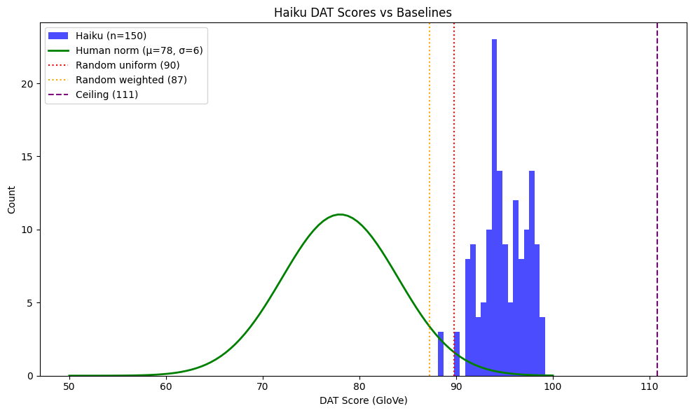Figure 4: Haiku DAT scores using GloVe embeddings compared to human norms and random baselines. Haiku’s distribution (blue, μ=94.8) is entirely disjoint from human norms (green, μ=78) and barely exceeds the random uniform baseline (red dotted, 90). This demonstrates that GloVe embeddings lack discriminative power for LLM-generated content.

4.3 Embedding Model Effects

The choice of embedding model dramatically affects scores:

Comparison	Value
GloVe mean	94.8
OpenAI mean	74.1
Difference	20.7 points
Correlation	r = 0.60

The moderate correlation (r = 0.60) confirms these embedding spaces capture different similarity structures. Scores are not interchangeable across models.

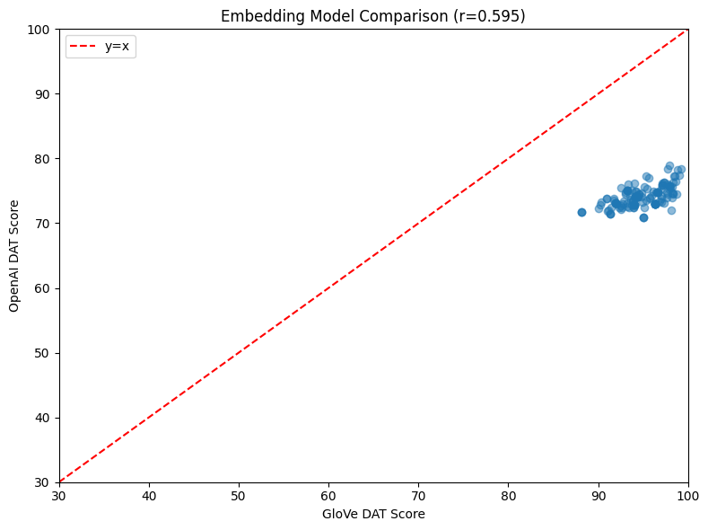Figure 5: GloVe vs OpenAI DAT scores across 150 trials. The 20.7-point systematic difference and moderate correlation (r = 0.60) demonstrate that embedding model choice fundamentally affects score interpretation.

Recommendation: Use OpenAI text-embedding-3-small as the standard embedding model. GloVe embeddings lack discriminative power for LLM-generated content.

4.4 Temperature Effects

Temperature	Mean Score	SD
0.0	73.8	1.4
0.5	74.2	1.6
1.0	74.3	1.8

Linear regression: R² = 0.006, p = 0.33

Finding: Temperature has negligible effect on divergent association capacity, simplifying deployment.

4.5 Calibration Adjustments

To convert INS-001 spread to DAT-equivalent scale:

Task	Haiku INS-001	Haiku DAT	Adjustment
INS-001.1	65.5	74.1	+8.6
INS-001.2 (overall)	66.1	74.1	+8.0
INS-001.2 (easy pairs)	63.8	74.1	+10.4
INS-001.2 (hard pairs)	67.6	74.1	+6.5

Note: INS-001.2 adjustments are stratified by pair difficulty because anchor-target distance moderates achievable spread.

4.6 Calibration Assumption Validation

The calibration assumes Haiku’s divergent capacity is constant across tasks—that score differences reflect task structure, not ability differences. We tested this by comparing pairwise distances:

Comparison	DAT Pairs	Bridging Clue Pairs
N pairs	3,150	5,202
Mean distance	0.741	0.654
SD	0.061	0.104

Statistical test: t = 42.6, p < 0.0001, Cohen’s d = 1.02 (large effect)

Warning: The assumption was not validated. DAT pairwise distances are systematically higher than bridging clue distances, even for the same model. This large effect (d = 1.02) indicates the bridging constraint genuinely compresses Haiku’s associative range—not just an artifact of pair composition.

Implication: The calibration adjustment accounts for this compression, but users should understand that constrained association (INS-001.2) produces systematically lower divergence than free association (DAT or INS-001.1) for fundamental geometric reasons, not just task structure.

---

5. INS-001.1: Radiation (Free Association)

5.1 Task Description

Participants receive a seed word and generate free associations. The task measures divergent thinking with an implicit constraint: associations should be recoverable by an external guesser.

Component	Description
Input	Single seed word
Output	2–10 association words
Constraint	Implicit (communicability)
Scoring	Spread + Communicability

5.2 Communicability Metric

Communicability measures whether a standardized guesser (Claude Haiku 4.5) can recover the original seed from the participant’s associations.

Protocol:

1. Present clues to Haiku (without seed)
2. Haiku generates top-3 guesses for the seed
3. Score as communicable if seed appears in guesses

Scoring:

• Exact match: Seed word appears verbatim
• Semantic match: Seed’s nearest neighbor in embedding space appears

5.3 Unconventionality Metric

Unconventionality measures how predictable a participant’s associations are—whether they avoided the obvious, “first thing that comes to mind” responses.

Rationale: High spread alone doesn’t distinguish between genuinely creative associations and merely random ones. Unconventionality captures whether participants explored outside the predictable semantic neighborhood, not just whether their words were distant from each other.

Algorithm:

def calculate_unconventionality(
    user_associations: list[str],
    noise_floor: list[str]  # Most predictable associations for seed
) -> dict:
    """
    Compare user associations against the predictable neighborhood.

    The noise floor contains the N most common/predictable associations
    for the seed word (e.g., nearest neighbors in embedding space,
    or empirically frequent human responses).
    """

    def is_match(user_word: str, floor_word: str) -> bool:
        """Check exact match or morphological variants."""
        # Normalize: lowercase, stem
        user_stem = stem(user_word.lower())
        floor_stem = stem(floor_word.lower())
        return user_stem == floor_stem

    # Count overlaps with noise floor
    overlaps = []
    for user_word in user_associations:
        for floor_word in noise_floor:
            if is_match(user_word, floor_word):
                overlaps.append(user_word)
                break

    overlap_count = len(overlaps)

    # Classify unconventionality
    if overlap_count == 0:
        level = "high"
        description = "None of your associations appeared in the predictable neighborhood."
    elif overlap_count <= 2:
        level = "moderate"
        description = f"{overlap_count} of your associations appeared in the predictable neighborhood."
    else:
        level = "low"
        description = f"{overlap_count} of your associations appeared in the predictable neighborhood."

    return {
        "level": level,
        "overlap_count": overlap_count,
        "overlapping_words": overlaps,
        "description": description
    }

Interpretation:

Overlap Count	Level	Interpretation
0	High	Avoided all predictable associations—genuinely unconventional
1–2	Moderate	Some predictable choices, but explored beyond the obvious
3+	Low	Most associations were predictable/conventional

Relationship to Other Metrics:

Unconventionality is distinct from both spread and communicability:

Metric	What It Measures	High Score Means
Spread	Distance between associations	Words are semantically far apart
Unconventionality	Distance from predictable set	Words avoided the obvious choices
Communicability	Guesser recovery success	Associations decode to correct seed

A participant could have:

• High spread + Low unconventionality: Words are distant from each other but all predictable (e.g., for “dog”: cat, bark, leash, walk)
• Low spread + High unconventionality: Words cluster together but in an unexpected region (e.g., for “dog”: loyalty, companionship, devotion)
• High spread + High unconventionality: The ideal—exploring distant, non-obvious territory

5.4 The Spread-Communicability Synergy

Contrary to expectation, spread and communicability show positive correlation:

Statistic	Value
Point-biserial correlation	r = 0.34, p < 0.0001
Communicable trials spread	66.0
Non-communicable trials spread	59.6
t-test	t = 6.40, p < 0.0001

Interpretation: Associations that are too constrained (low spread) may be idiosyncratic and fail to communicate. Moderate divergence appears optimal—it provides multiple triangulation points without becoming disconnected from the seed.

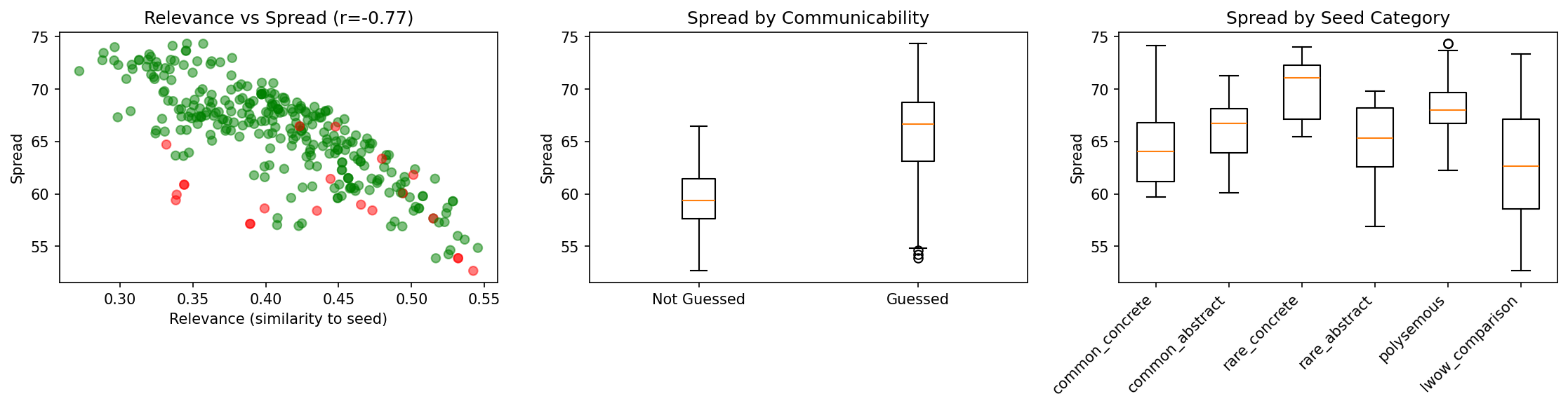Figure 1: INS-001.1 calibration results. Left: Spread-relevance inverse correlation (r = -0.77), with green points showing communicable trials and red showing non-communicable. Middle: Spread distribution by communicability status—communicable trials show higher spread (the synergy). Right: Spread varies by seed category, with rare concrete words producing highest spread.

5.5 Spread-Relevance Relationship

The strong inverse correlation between spread and relevance (r = -0.77) confirms these measure the same dimension from opposite poles:

Spread Quartile	Relevance Mean	Communicability
Q1 (low)	0.47	78.2%
Q2	0.42	97.4%
Q3	0.40	97.4%
Q4 (high)	0.36	100%

Higher spread → lower relevance → higher communicability. The “conventional” associations (high relevance, low spread) are actually harder to decode.

5.6 Optimal Clue Count

Clues	Spread	SD	Communicability
1	—	—	100%
2	69.7	8.6	100%
3	68.1	6.2	100%
5	65.4	4.9	100%
10	66.6	4.4	100%

Recommendation: 2 clues—maximum spread while maintaining perfect communicability.

Figure 2: INS-001.1 metrics by clue count. Top-left: Spread decreases then stabilizes as clues increase. Top-right: Communicability remains at ceiling across all clue counts. Bottom-left: Spread vs communicability shows all configurations above 80% threshold. Bottom-right: Relevance decreases slightly with more clues.

5.7 Seed Category Effects

Category	Spread	Relevance	Communicability
Common concrete	64.7	0.422	100%
Common abstract	65.9	0.433	100%
Rare concrete	69.9	0.331	100%
Rare abstract	65.0	0.417	100%
Polysemous	68.3	0.391	100%

ANOVA for spread: F = 19.96, p < 0.0001

Finding: Rare concrete words produce highest spread—likely because they have fewer strong associates, forcing exploration.

5.8 Haiku Version Comparison

Comparing Haiku 3.5 (from LWOW dataset) to Haiku 4.5:

Metric	Value
Mean Jaccard similarity	0.213
Mean overlap (of 3 clues)	0.95
Perfect match rate	0%
No overlap rate	25%

Interpretation: Haiku versions share some associations but are not identical. Model version should be locked for reproducibility.

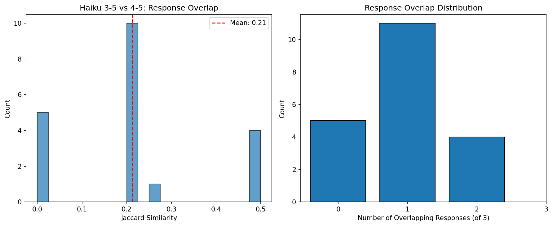Figure 3: Association overlap between Haiku 3.5 and 4.5 across 20 seed words.

---

6. INS-001.2: Bridging (Constrained Association)

6.1 Task Description

Participants receive an anchor-target word pair and generate clues that connect them. The task measures divergent thinking with an explicit geometric constraint.

Component	Description
Input	Anchor word + Target word
Output	4–5 clue words
Constraint	Explicit (must bridge)
Scoring	Spread + Fidelity

6.2 Fidelity Metric

Fidelity measures how well clues collectively identify the anchor-target pair by eliminating plausible alternatives.

Intuition: Good bridging clues should:

• Coverage: Eliminate most alternative endpoints (each clue rules out some wrong answers)
• Efficiency: Be non-redundant (different clues eliminate different wrong answers)

Bad clues either:

• Eliminate nothing (uninformative—too far from endpoints)
• All eliminate the same foils (redundant—no complementary information)

6.2.1 Mathematical Formulation

Let $\mathbf{a}$ be the anchor embedding, $\mathbf{t}$ the target embedding, and $\{\mathbf{c}_1, ..., \mathbf{c}_n\}$ the clue embeddings.

Foil sets: For each endpoint, generate the 50 nearest neighbors in embedding space:

• $F_a = \{f_1^a, ..., f_{50}^a\}$ — foils for anchor
• $F_t = \{f_1^t, ..., f_{50}^t\}$ — foils for target

Elimination: A clue $\mathbf{c}_i$ eliminates foil $f_j$ if the clue is more similar to the true endpoint than to the foil:

$$\text{eliminates}(\mathbf{c}_i, f_j^a) = \mathbb{1}\left[\cos(\mathbf{c}_i, \mathbf{a}) > \cos(\mathbf{c}_i, f_j^a)\right]$$

Elimination sets: For each clue, compute the set of foils it eliminates:

$$E_i^a = \{j : \text{eliminates}(\mathbf{c}_i, f_j^a)\}$$

Coverage: Fraction of foils eliminated by at least one clue:

$$\text{coverage}_a = \frac{|\bigcup_{i=1}^{n} E_i^a|}{|F_a|}$$

Efficiency: Non-redundancy of elimination (1 minus the Jaccard-like redundancy):

$$\text{efficiency}_a = 1 - \frac{|\bigcap_{i=1}^{n} E_i^a|}{|\bigcup_{i=1}^{n} E_i^a|}$$

Combined fidelity:

$$\text{fidelity} = \frac{\text{coverage}_a + \text{coverage}_t}{2} \times \frac{\text{efficiency}_a + \text{efficiency}_t}{2}$$

6.2.2 Algorithm Implementation

def calculate_fidelity(
    clue_embeddings: list[list[float]],
    anchor_embedding: list[float],
    target_embedding: list[float],
    foil_anchors: list[list[float]],  # 50 nearest neighbors of anchor
    foil_targets: list[list[float]],  # 50 nearest neighbors of target
) -> dict:
    """
    Measure how well clues jointly constrain the solution space.

    A foil is "eliminated" by a clue if that clue is more similar to the
    true endpoint than to the foil.
    """

    def get_eliminations(clue_emb, true_emb, foil_embs):
        """Return set of foil indices eliminated by this clue."""
        true_sim = cosine_similarity(clue_emb, true_emb)
        eliminated = set()
        for i, foil in enumerate(foil_embs):
            foil_sim = cosine_similarity(clue_emb, foil)
            if true_sim > foil_sim:
                eliminated.add(i)
        return eliminated

    # Compute eliminations for each clue
    anchor_elims = [get_eliminations(c, anchor_embedding, foil_anchors)
                    for c in clue_embeddings]
    target_elims = [get_eliminations(c, target_embedding, foil_targets)
                    for c in clue_embeddings]

    # Coverage: fraction of foils eliminated by at least one clue
    anchor_union = set.union(*anchor_elims) if anchor_elims else set()
    target_union = set.union(*target_elims) if target_elims else set()
    anchor_coverage = len(anchor_union) / len(foil_anchors)
    target_coverage = len(target_union) / len(foil_targets)

    # Efficiency: 1 - (intersection / union)
    def compute_efficiency(elim_sets):
        if len(elim_sets) < 2:
            return 1.0
        union = set.union(*elim_sets)
        if not union:
            return 0.0
        intersection = set.intersection(*elim_sets)
        redundancy = len(intersection) / len(union)
        return 1 - redundancy

    anchor_efficiency = compute_efficiency(anchor_elims)
    target_efficiency = compute_efficiency(target_elims)

    # Combined metrics
    overall_coverage = (anchor_coverage + target_coverage) / 2
    overall_efficiency = (anchor_efficiency + target_efficiency) / 2
    fidelity = overall_coverage * overall_efficiency

    return {
        "fidelity": fidelity,
        "coverage": overall_coverage,
        "efficiency": overall_efficiency
    }

6.2.3 Foil Generation

Foils are the 50 nearest neighbors of each endpoint in embedding space:

def generate_endpoint_foils(
    endpoint_embedding: list[float],
    vocabulary_embeddings: dict[str, list[float]],
    n_foils: int = 50
) -> list[list[float]]:
    """
    Generate hard-to-distinguish foils using nearest neighbors.
    """
    vocab_embs = list(vocabulary_embeddings.values())
    similarities = [cosine_similarity(endpoint_embedding, v) for v in vocab_embs]
    sorted_indices = np.argsort(similarities)[::-1]
    # Skip index 0 (might be the word itself)
    foil_indices = sorted_indices[1:n_foils+1]
    return [vocab_embs[i] for i in foil_indices]

Why nearest neighbors? These are the hardest foils to distinguish—words semantically similar to the true endpoint. If clues can eliminate these, they carry strong signal about the true pair.

6.2.4 Component Interpretation

Component	Meaning	Low Value	High Value
Coverage	Fraction of foils eliminated	Clues too distant from endpoints	Clues in right neighborhood
Efficiency	Non-redundancy of elimination	All clues eliminate same foils	Complementary information

Both components contribute to fidelity. A score can be high-coverage but low-efficiency (redundant conventional clues) or low-coverage but high-efficiency (sparse but complementary).

6.3 Why Fidelity Replaced Relevance

The original relevance metric exhibited a strong inverse correlation with spread:

Issue	Relevance	Fidelity
Spread correlation	r = -0.61 (redundant)	r = +0.06 (independent)
A-T distance correlation	r = -0.41 (confounded)	r = +0.02 (unconfounded)
Interpretation	”How close to corridor"	"How well do clues triangulate”

The fundamental tradeoff: Trial-level correlation between relevance and clue-only divergence was r = -0.61 (p < 0.0001). This is geometric—clues close to both endpoints must cluster together.

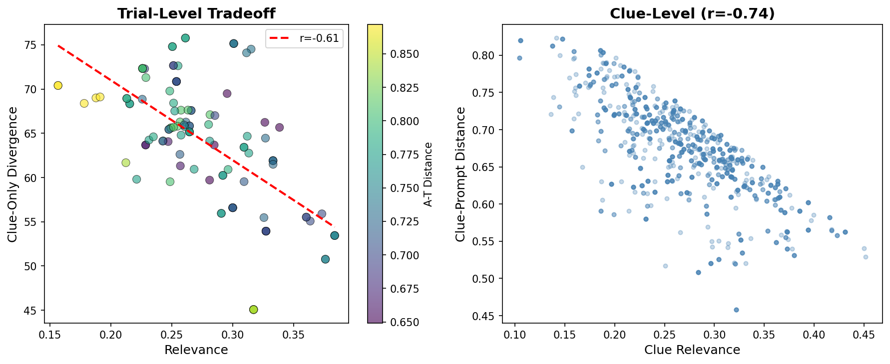Figure 7: The relevance-divergence tradeoff in INS-001.2. Left: Trial-level correlation (r = -0.61) between relevance and clue-only divergence, with points colored by anchor-target distance. Right: Clue-level correlation (r = -0.74) showing that more relevant clues are closer to the prompt words.

Fidelity was selected from three candidate metrics based on: lowest spread correlation, lowest difficulty confound, no ceiling effect, and interpretable decomposition (coverage × efficiency).

6.4 Pair Difficulty Moderation

Anchor-target distance affects achievable spread—a key moderating variable for interpretation.

Difficulty	A-T Distance	Clue-Clue Spread	N
Easy	0.696	63.8 ± 3.9	39
Medium	0.754	64.8 ± 4.6	38
Hard	0.811	67.6 ± 4.4	39

ANOVA: F = 8.08, p = 0.0005, η² = 0.13 (medium effect)

Post-hoc comparisons (Bonferroni-corrected):

• Easy vs Hard: Δ = -3.80, p = 0.0001 ***
• Medium vs Hard: Δ = -2.71, p = 0.010 *
• Easy vs Medium: Δ = -1.10, p = 0.26 (ns)

Interpretation: When endpoints are farther apart, there’s more geometric “room” for clue spread without violating relevance constraints. This 3.8-point difference between easy and hard pairs is substantial—nearly one standard deviation.

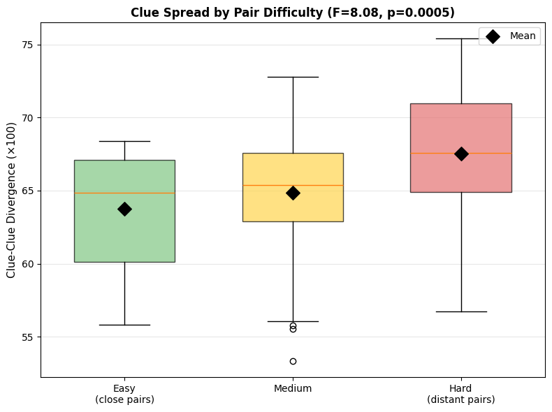Figure 8: Clue-clue spread by pair difficulty tercile. Harder pairs (greater A-T distance) allow significantly more spread.

Implication: INS-001.2 scores should be interpreted relative to pair difficulty. A spread of 65 on an easy pair reflects more divergent capacity than 65 on a hard pair. Stratified calibration adjustments account for this:

Difficulty	A-T Threshold	DAT Adjustment
Easy	< 0.727	+10.4 points
Medium	0.727–0.777	+9.3 points
Hard	> 0.777	+6.5 points

6.5 Optimal Clue Count

Spread stabilizes after 3–4 clues, with diminishing marginal contribution:

Clues	Full Spread	SD	Clue-Clue Pairs	Gap to DAT
1	68.6	5.2	0	+5.5
2	66.8	5.1	1	+7.3
3	66.4	4.8	3	+7.7
4	66.3	4.7	6	+7.8
5	66.2	4.7	10	+7.9
10	66.2	4.1	45	+7.9

Marginal contribution analysis: After 2 clues, additional clues provide negligible marginal divergence (all p > 0.05 except 1→2 which shows Δ = -1.85, p < 0.0001).

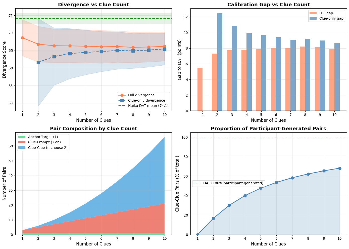Figure 9: INS-001.2 divergence trajectories by clue count. Top-left: Full and clue-only divergence converge as clue count increases. Top-right: Gap to DAT stabilizes around 8 points. Bottom-left: Pair composition shifts toward clue-clue pairs. Bottom-right: Proportion of participant-generated pairs increases but never reaches DAT’s 100%.

Optimization criteria:

1. Gap to DAT (construct validity)
2. Clue-clue pair proportion (purity of divergence measurement)
3. Score stability (SD)
4. Task efficiency (participant burden)

Recommendation: 4 clues—balances construct validity (40% clue-clue pairs), stability (SD = 4.7), and reasonable task length.

6.6 Joint Interpretation

Spread	Fidelity	Interpretation
High	High	Creative and precise bridging
High	Low	Divergent but off-task
Low	High	Conventional but effective
Low	Low	Constrained and off-task

---

7. Interpretation Thresholds

7.1 INS-001.1 Spread Thresholds (Haiku-Calibrated)

Score	Label	Description	Haiku Percentile
< 59	Low	Very constrained associations	< 10th
59–62	Below Average	Limited exploration	10th–25th
62–69	Average	Typical free association	25th–75th
69–72	Above Average	Wide-ranging associations	75th–90th
> 72	High	Exceptional spread	> 90th

Haiku reference: mean = 65.5, SD = 4.6

7.2 INS-001.1 Unconventionality Thresholds

Overlap Count	Level	Interpretation
0	High	Fully avoided predictable associations
1–2	Moderate	Partial exploration beyond the obvious
3+	Low	Relied on predictable/conventional associations

Note: Unconventionality should be interpreted alongside spread and communicability. The ideal profile is high spread + high unconventionality + successful communicability—exploring distant, non-obvious territory while still communicating effectively.

7.3 INS-001.1 Communicability Expectations

Rate	Interpretation
< 80%	Idiosyncratic associations—may not communicate
80–90%	Partial communication—some unusual associations
> 90%	Effective communication—associations decode reliably

Haiku reference: 93.2%

7.4 INS-001.2 Spread Thresholds (Haiku-Calibrated)

Score	Label	Description	Haiku Percentile
< 55	Low	Very constrained associations	< 5th
55–62	Below Average	Limited exploration	5th–25th
62–68	Average	Typical bridging performance	25th–75th
68–72	Above Average	Wide-ranging associations	75th–95th
> 72	High	Exceptional spread	> 95th

Haiku reference: mean = 64.4, SD = 4.6

7.5 INS-001.2 Fidelity Thresholds (Haiku-Calibrated)

Score	Label	Description	Haiku Percentile
< 0.50	Diffuse	Clues don’t narrow down the connection	< 5th
0.50–0.65	Partial	Some constraint, with redundancy	5th–25th
0.65–0.75	Moderate	Reasonable triangulation	25th–75th
0.75–0.85	Focused	Efficient identification	75th–95th
> 0.85	Precise	Optimal constraint	> 95th

Haiku reference: mean = 0.68, SD = 0.13

7.6 DAT-Equivalent Conversion

To express INS-001 spread in DAT-equivalent terms:

Original	Adjustment	DAT-Equivalent	Interpretation
INS-001.1: 60	+8.6	68.6	Below human average
INS-001.1: 65	+8.6	73.6	Near human average
INS-001.1: 70	+8.6	78.6	At human average
INS-001.2: 60	+9.7	69.7	Below human average
INS-001.2: 65	+9.7	74.7	Near human average

Human DAT reference: mean = 78, SD = 6

---

8. Implementation

8.1 Core Functions

Function	INS-001.1	INS-001.2
calculate_spread()	✓	✓
calculate_unconventionality()	✓	—
calculate_communicability()	✓	—
calculate_fidelity()	—	✓
generate_endpoint_foils()	—	✓
generate_noise_floor()	✓	—
score_radiation()	✓	—
score_bridging()	—	✓

8.2 Return Schemas

INS-001.1 (score_radiation()):

{
    "spread": float,              # Clue-only divergence (0-100)
    "relevance": float,           # Legacy metric (0-1)
    "communicable": bool,         # Did Haiku guess correctly?
    "haiku_guesses": list,        # Top-3 guesses
    "exact_match": bool,          # Verbatim match
    "semantic_match": bool,       # Nearest-neighbor match
    "unconventionality": {
        "level": str,             # "high", "moderate", or "low"
        "overlap_count": int,     # Number of predictable associations
        "overlapping_words": list # Which words matched noise floor
    }
}

INS-001.2 (score_bridging()):

{
    "spread": float,              # Clue-only divergence (0-100)
    "fidelity": float,            # Joint constraint score (0-1)
    "fidelity_coverage": float,   # Coverage component (0-1)
    "fidelity_efficiency": float, # Efficiency component (0-1)
    "relevance": float,           # Legacy metric (0-1)
    "valid": bool                 # Whether relevance >= 0.15
}

8.3 Dependencies

Component	Specification
Embedding model	OpenAI text-embedding-3-small (1536 dim)
Guesser model	Claude Haiku 4.5 (claude-haiku-4-5-20251001)
Vocabulary	~5000 common English nouns
Foil count	50 per endpoint

8.4 Computational Cost

Operation	INS-001.1	INS-001.2
Embeddings	O(n) clues	O(n) clues
Spread	O(n²) pairs	O(n²) pairs
Fidelity	—	O(n × 100) foils
Guesser call	1 API call	—

---

9. Limitations

Limitation	Impact	Mitigation
Haiku as reference	AI may not match human associations	Plan human validation study
Embedding dependence	Different models yield different scores	Standardize on OpenAI; re-calibrate if changed
Cultural bias	Semantic structures vary by culture/language	Document English-only scope; expand later
Guesser brittleness	Haiku capabilities may shift	Lock model version; re-calibrate periodically
Single-trial reliability	High variance per trial	Use multiple trials; report aggregates

---

10. Code

Implementation available at:

• Scoring module: scoring.py

---

Changelog

Version	Date	Changes
4.0	2026-01-18	Expanded scope to cover both INS-001.1 and INS-001.2; added theoretical framework on semantic memory and communication fidelity; added INS-001.1 calibration study with spread-communicability synergy finding; added DAT calibration details including embedding model effects; documented optimal clue counts for both instruments
3.0	2026-01-18	Replaced relevance with fidelity for INS-001.2; added fidelity calibration study
2.0	2026-01-17	Added DAT calibration; renamed “divergence” to “spread”
1.0	2026-01-15	Initial publication

---

Figures

The following figures are referenced in this document (located in /images/methods/semantic-association-metrics/spread-fidelity-scoring/):

INS-001.1 (Radiation):

1. ins001_1_calibration.png — Spread-relevance relationship and seed category effects
2. ins001_1_clue_count_trajectories.png — Spread and communicability by clue count
3. ins001_1_haiku_version_comparison.png — Association overlap between Haiku versions

DAT Calibration: 4. dat_scores_vs_baselines.png — Haiku vs human norms vs random baselines 5. embedding_model_comparison.png — GloVe vs OpenAI DAT score comparison

INS-001.2 (Bridging): 6. alternative_relevance_metrics.png — Fidelity metric selection analysis 7. relevance_divergence_tradeoff.png — The fundamental relevance-spread tradeoff 8. pair_difficulty_moderation.png — Clue spread by pair difficulty tercile 9. divergence_trajectory.png — Full and clue-only divergence by clue count 10. tercile_comparison.png — Fidelity by spread tercile 11. metric_correlations.png — Correlation heatmap for all INS-001.2 metrics